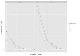
Stata Zero Inflated Negative Binomial

Stata Zero Inflated Negative Binomial, model is a type of count data regression model designed to handle datasets where:

1. There are excess zero counts (more zeroes than would be expected in a standard negative binomial distribution).
2. The counts that do occur exhibit overdispersion (the variance exceeds the mean, which is common in real-world count data).

To address these two issues, the ZINB model combines two components:

• A count model (in this case, the negative binomial distribution) that models the non-zero counts.
• A binary model (usually a logit or probit model) that models the probability of an observation being a zero.

Thus, the ZINB model assumes that there are two distinct processes generating the observed data:

1. A structural process that generates excessive zero counts (e.g., some observations are always zero due to an underlying condition).
2. A count process that generates the non-zero counts based on the negative binomial distribution.

The Negative Binomial distribution is often used in count data models when the data exhibit overdispersion (i.e., the variance is greater than the mean), which is a limitation of the Poisson distribution. The Zero-Inflated part of the model accounts for the extra zeros by using a binary model to determine whether an observation will result in a zero or a count.

When to Use a Zero-Inflated Negative Binomial Model

The ZINB model is particularly useful in the following situations:

• Excessive Zeros: You have a count variable where zero counts occur more often than the standard Poisson or Negative Binomial models can explain. For example, in a study of hospital visits, many people may not visit the hospital at all, leading to an excess of zero counts.
• Overdispersion: Your count data shows overdispersion, where the variance is significantly larger than the mean. This violates the assumption of the Poisson model, where the mean and variance are assumed to be equal.

Some common examples of data that may require a ZINB model include:

• Insurance claim data, where most policyholders have no claims, but a small number make frequent claims.
• Ecological studies, where most species in a region may be absent, but a few are abundant.
• Crime data, where many areas may have no reported crimes, but certain areas have frequent incidents.

Fitting the ZINB Model in Stata

In Stata, the ZINB model can be estimated using the zinb command. Here’s the general syntax:

Where:

• depvar is the dependent variable (the count variable).
• indepvars are the independent variables that influence the count process.
• inflate(inflation_vars) specifies the independent variables that influence the zero-inflation process.

Example: Fitting a ZINB Model in Stata

Let’s say you are analyzing the number of doctor visits (doctor_visits) in a dataset where individuals may either make no visits at all (excess zeroes) or a small number of visits, but there’s significant overdispersion in the count data. You want to model the count data based on age and income, while accounting for the probability of being a non-visiting individual (i.e., zero inflation) using education level.

Here’s how you would run the ZINB model in Stata:

In this case:

• The count process is modeled by doctor_visits as a function of age and income.
• The zero-inflation process is modeled by education, which affects the likelihood of making zero visits.

Interpreting the Results

When you run the zinb command, Stata provides two sets of results:

1. The count model coefficients (the part of the model that explains the non-zero counts).
2. The zero-inflation model coefficients (the part of the model explaining why some observations are always zero).

• Count model coefficients: These are interpreted like the coefficients in a standard negative binomial regression. For example, a positive coefficient for age would indicate that older individuals are more likely to have a higher number of doctor visits, assuming no excess zeros are involved.
• Zero-inflation model coefficients: These coefficients explain the likelihood that an observation is an “excess zero.” For example, if education has a negative coefficient, it would suggest that higher levels of education are associated with a lower probability of reporting zero doctor visits.

Both models work together to give a fuller picture of the underlying data structure—accounting for both the excess zeros and the overdispersion in the counts.

Model Diagnostics and Goodness of Fit

After fitting a ZINB model, it’s important to assess its fit and validity. Some common steps include:

• Checking for overdispersion: Compare the ZINB model to the standard Poisson or negative binomial models using likelihood ratio tests or Vuong’s test to determine if the ZINB model is indeed a better fit for your data.
• Goodness-of-Fit Tests: Use estat gof to conduct goodness-of-fit tests to assess the adequacy of your model.
• Model Comparisons: Compare the ZINB model with other zero-inflated models, such as the Zero-Inflated Poisson (ZIP) model, to determine which model better fits your data.

Limitations and Considerations

While the ZINB model is powerful, it’s not without limitations:

1. Model Complexity: The ZINB model involves two separate processes, making it more complex to estimate and interpret than simpler models like Poisson regression.
2. Collinearity: As with any regression model, you must be cautious about collinearity between predictors, especially in the zero-inflation component, where multicollinearity can distort results.
3. Large Sample Size: Like many complex models, the ZINB requires a large sample size to produce reliable estimates.

Conclusion

The Zero-Inflated Negative Binomial (ZINB) model is an essential tool for handling count data that exhibits both excess zero counts and overdispersion. Stata’s implementation of the ZINB model allows researchers to model such data with ease, providing a more accurate representation of the underlying data-generating processes.

By properly specifying the two components (the count process and the zero-inflation process), you can obtain more reliable and interpretable results, especially in fields like economics, epidemiology, and social sciences. However, careful diagnostic testing and model comparison are crucial to ensure the robustness and reliability of your findings.

If your data features these complexities, the ZINB model in Stata could be just what you need to unlock the insights you’re looking for.